Image Segmentation - K-Means Clustering
Published:
Contents
- K-means (pixel-wise) segmentation
- Chan-Vese (region-wise) segmentation
K-Means Segmentation
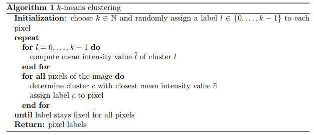
K-Means is a well-known algorithm for clustering, most often applied to tabular data in unsupervised learning. However, an interesting application is pixel-wise Image Segmentation.
The method involves dividing the image into \(k\) clusters based on pixel intensity values. Each pixel is assigned a label corresponding to its cluster. This process iteratively minimizes the within-cluster variance.
Mathematical Explanation
K-Means clustering seeks to minimize the following objective function: \(J = \sum_{i=1}^{k} \sum_{x \in C_i} \ \vert x - \mu_i\ \vert ^2,\) where:
- \(k\) is the number of clusters,
- \(C_i\) is the set of pixels in the \(i\)-th cluster,
- \(\mu_i\) is the mean intensity value of the \(i\)-th cluster,
- \(\ \vert x - \mu_i\ \vert ^2\) represents the squared Euclidean distance between a pixel \(x\) and the cluster mean.
The algorithm alternates between two steps:
- Assignment Step: Assign each pixel to the nearest cluster mean: \(c(x) = \arg\min_{i} \ \vert x - \mu_i\ \vert ^2.\)
- Update Step: Recompute the cluster means based on the new assignments: \(\mu_i = \frac{1}{ \vert C_i \vert } \sum_{x \in C_i} x.\) The algorithm terminates when cluster assignments no longer change.
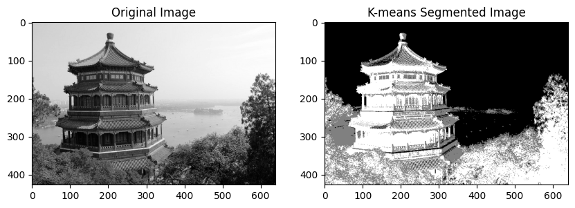
Implementation - K-Means Segmentation
from __future__ import annotations
import os
from PIL import Image
import numpy as np
import matplotlib.pyplot as plt
import cv2
from sklearn.datasets import load_sample_image
import numpy as np
import matplotlib.pyplot as plt
from sklearn.datasets import load_sample_image

def k_means_clustering(f, k):
  if k is None:
    k = np.random.randint(0, 10)

  rows, cols = f.shape # image shape
  labels = np.random.randint(0, k, (rows, cols))  # Random initial labels
  cluster_centers = np.zeros(k)

  while True:
    # compute cluster centers
    for i in range(k):
      cluster_centers[i] = np.mean(f[labels == i])

    # assign pixels to the closest cluster center
    new_labels = np.zeros((rows, cols), dtype=int)
    for i in range(rows):
      for j in range(cols):
        new_labels[i, j] = np.argmin(np.abs(cluster_centers - f[i, j]))

    # check for convergence
    if np.array_equal(new_labels, labels):
      break

    labels = new_labels

  return labels

def run_kmeans_segmentation(image, k=3):
  grayscale_image = np.mean(image, axis=2)  # Convert to grayscale

  labels = k_means_clustering(grayscale_image, k)

  # Display the original image and the segmented image
  plt.figure(figsize=(10, 5))
  plt.subplot(1, 2, 1)
  plt.imshow(grayscale_image, cmap='gray')
  plt.title('Original Image')

  plt.subplot(1, 2, 2)
  plt.imshow(labels, cmap='gray')
  plt.title('K-means Segmented Image')
  plt.show()
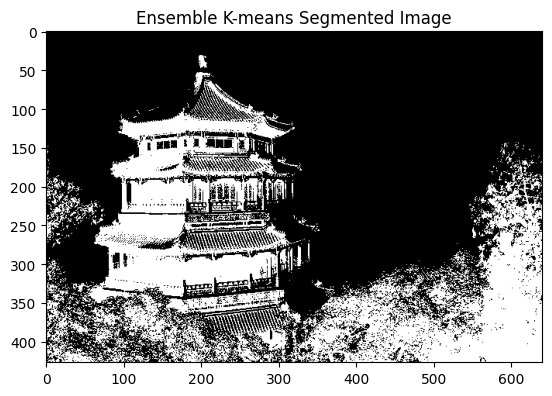
Ensemble K-Means Segmentation
In cases where K-Means clustering may be sensitive to initialization, an ensemble method can stabilize results. The ensemble approach runs the K-Means algorithm multiple times and combines the results using majority voting for each pixel.
Implementation
def k_means_ensemble(f, k, repetitions):
    # Input:
    # f - grayscale image matrix
    # k - number of clusters
    # repetitions - number of k-means runs
    # Output:
    # labels - matrix with the same size as f containing the combined cluster labels

    # Initialize variables
    rows, cols = f.shape
    votes = np.zeros((rows, cols, repetitions), dtype=int)

    # Run k-means clustering multiple times
    for r in range(1, repetitions+1):
        print('repetion: {}/{} ({:.3f}%)'.format(r, repetitions,
                                               r*100/repetitions))
        votes[:, :, r-1] = k_means_clustering(f, k)

    # Combine the results using majority voting
    labels = np.zeros((rows, cols), dtype=int)
    for i in range(rows):
        for j in range(cols):
            labels[i, j] = np.bincount(votes[i, j, :]).argmax()  # Majority voting

    return labels

def run_kmeans_ensemble(image,
                        k=3,
                        repetitions = 10):
  grayscale_image = np.mean(image, axis=2)  # Convert to grayscale

  ensemble_labels = k_means_ensemble(grayscale_image, k, repetitions)

  # Display the ensemble segmented image
  plt.figure()
  plt.imshow(ensemble_labels, cmap='gray')
  plt.title('Ensemble K-means Segmented Image')
  plt.show()
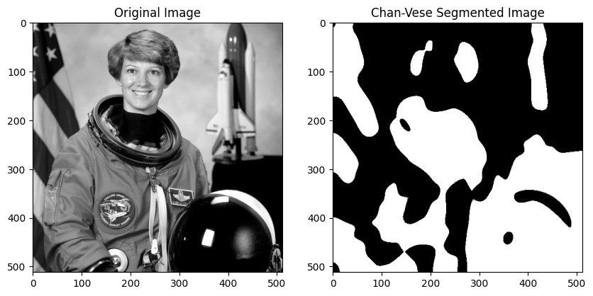
Chan-Vese Segmentation
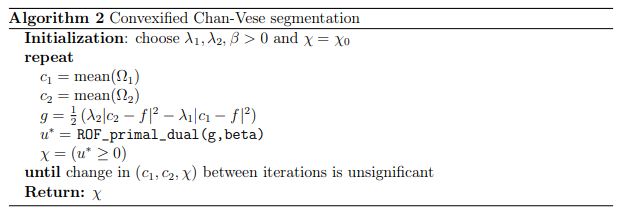
A popular region-based segmentation method is the Chan-Vese model, which seeks to partition the image domain \(\Omega \subset \mathbb{R}^d\) into regions of approximately constant intensity. The domain is encoded by an indicator function \(\chi\) by approximating the given image f with constant functions \(c_1, c_2 \in \mathbb{R}\), i.e.,
\begin{split} \min_{c_1,c_2, \chi \in BV(\Omega, {0,1})} J(c_1,c_2, \chi)= & \frac{\lambda_1}{2} \int_{\Omega} \chi \vert c_1-f(x) \vert ^2dx
& +\frac{\lambda_2}{2} \int_{\Omega} (1 - \chi) \vert c_2-f(x) \vert ^2dx & +\beta \vert \chi \vert _{BV} \end{split}
for which \(\chi: \Omega \to \{0, 1\}\) is the indicator function given by: \(\chi(x) = \begin{cases}1 & \text{if } x \in \Omega_1 \\ 0 & \text{, else} \end{cases}\)
As the model in (1) is non-convex, we use an alternating minimization scheme for which one of the subproblems is a minimal surface problem, i.e.,
\[\min_{c_1,c_2, \chi \in BV(\Omega, \{0,1\})} J(c_1,c_2, \chi) = \int_{\Omega} \chi(x) \cdot \frac{1}{2}(\lambda_1 \vert c_1-f(x) \vert ^2 - \lambda_2 \vert c_2-f(x) \vert ^2 ) dx +\beta \vert \chi \vert _{BV}\]And note that \(g(x):=\frac{1}{2}( \lambda_1 \vert c_1-f(x) \vert ^2 - \lambda_2 \vert c_2-f(x) \vert ^2)dx\).
Note that this segmentation problem can be solved uniquely via a direct relationship to the ROF denoising model:
\[u^* = \arg\min_{u \in \Omega} J(u)\]with \(J(u) = \frac{1}{2} \ \vert u-g\ \vert ^2_{L^2(\Omega)} + \beta \vert u \vert _{BV}\)
Subsequently, we perform thresholding on \(u^∗\) at \(t = 0\) to obtain the solution \(\chi\). This convexified version of the Chan-Vese model can be implemented as follows.
Implementation
import numpy as np
import matplotlib.pyplot as plt
from skimage import color, data, img_as_float
from skimage.restoration import denoise_tv_chambolle

def chan_vese(f, lambda1, lambda2, beta, max_iter=100, tol=1e-3):
  # initialize chi with a checkerboard pattern
  chi = np.zeros_like(f, dtype=np.bool_)
  chi[::2, ::2] = 1
  chi[1::2, 1::2] = 1

  for _ in range(max_iter):
    # update c1 and c2
    c1 = np.mean(f[chi])
    c2 = np.mean(f[~chi])

    # compute the auxiliary function g
    g = 0.5 * (lambda2 * (c2 - f)**2 - lambda1 * (c1 - f)**2)

    # solve the ROF denoising problem (using total variation denoising)
    u_star = denoise_tv_chambolle(g, weight=beta, multichannel=False)

    # update chi
    chi_new = u_star >= 0

    # check for convergence
    if np.linalg.norm(chi_new.astype(int) - chi.astype(int)) < tol:
      break

    chi = chi_new

    return chi

def run_chan_vese(image, lambda1=1, lambda2=1, beta=0.1):
  image = color.rgb2gray(image)
  image = img_as_float(image)

  chi = chan_vese(image, lambda1, lambda2, beta)

  # Display the original image and the segmented image
  plt.figure(figsize=(10, 5))
  plt.subplot(1, 2, 1)
  plt.imshow(image, cmap='gray')
  plt.title('Original Image')

  plt.subplot(1, 2, 2)
  plt.imshow(chi, cmap='gray')
  plt.title('Chan-Vese Segmented Image')
  plt.show()

run_chan_vese(data.astronaut())
