Space Flight Trajectory prediction via Kalman-Filter
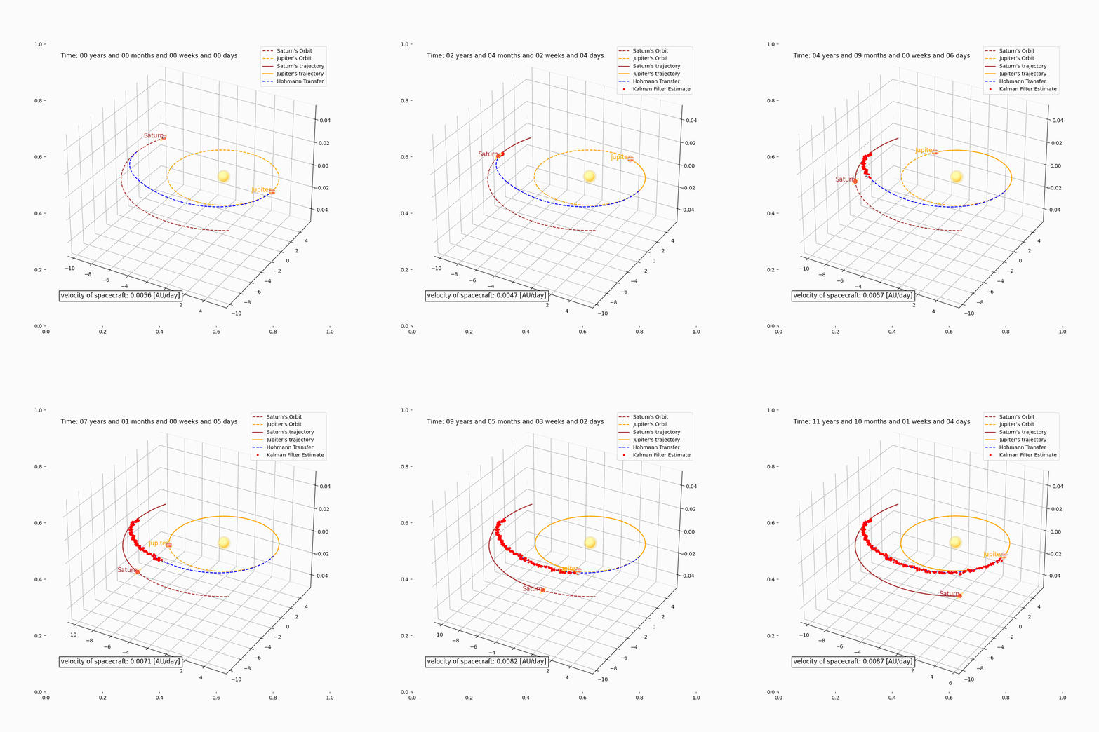
This project was presented for the Modeling Simulation and Optimization FAU Summer Semester 2024 master’s course.
The group modeled a space flight simulation between Saturn and Jupiter using the Hohmman Transfer theory and tools such as the Kalman-Filter model, to estimate trajectory states.
Simulation: Trajectory Prediction, Kalman-Filter
Motivation
- Why use the Kalman-Filter?
- Are the dynamics of our system (e.g. velocities) being considered?
- How do we account for noise and perturbations to our trajectory?
- How does NASA use the Kalman-Filter?
- Given a theoretical trajectory, does our spacecraft actually follow the trajectory?
- Are our assumptions viable?
How does NASA use the Kalman-Filter?
Applications:
- Navigation and guidance systems: real-time updates, combining data from inertial navigation systems and other sensors.
- Attitude estimation: used on the International Space Station (ISS), to fuse data from star trackers, gyroscopes, and other sensors, for the station orientation.
Examples:
- Apollo program.
- Mars Rover.
Kalman-Filter: Predicting the Next Position
Given observed positions, and taking into account the dynamics \((x, \dot{x}, \ddot{x})\), we want a method that can accurately estimate the next position, considering perturbations in our system.
Kalman-Filter: Embedding Uncertainty
- \(Q\): Process noise covariance, uncertainty about the system dynamics.
- \(R\): Measurement noise covariance.
- \(P\): Initial estimate covariance, uncertainty of initial estimate.
Kalman-Filter: Notation
- measurement at \(k-1\): \(\hat{x}_{k-1 \vert k-1}\)
- state update: \(\hat{x}_{k-1 \vert k-1} \to \hat{x}_{k \vert k-1}\)
- incorporate noise, updated covariance: \(\hat{x}_{k \vert k-1} \to \hat{x}_{k \vert k}\)
- measurement at \(k\): \(\hat{x}_{k \vert k}\)
Kalman Filter Algorithm Framework
- State update:
- Measurement update:
where we can abbreviate the factors:
- \[S = H P_{k \vert k-1} H^T + R\]
- \[y = z_k - H \hat{x}_{k \vert k-1}\]
Kalman-Filter: Estimation from Observed Measurements
To simulate observed measurements, we take the Hohmann transfer \(x_{h}, y_{h}\) vectors of positions and add a Gaussian noise with arbitrary variance \(\sigma^2\):
\[x_{\text{obs}} = x_{\text{Hohmann}} + n, \quad n \in \mathcal{N}(0, \sigma^2)\] \[y_{\text{obs}} = y_{\text{Hohmann}} + n, \quad n \in \mathcal{N}(0, \sigma^2)\]How does the Kalman-Filter takes into account the state?
Example with nonconstant velocity, and constant acceleration:
\[\begin{cases} \hat{x}_{k+1,k} = \hat{x}_{k,k} + \hat{\dot{x}}_{k,k} \Delta t + \frac{1}{2} \hat{\ddot{x}}_{k,k} \Delta t^2 \\ \hat{\dot{x}}_{k+1, k} = \hat{\dot{x}}_{k,k} + \hat{\ddot{x}}_{k,k} \Delta t \\ \hat{\ddot{x}}_{k+1, k} = \hat{\ddot{x}}_{k, k} \\ \end{cases}\]Then, the state update is:
\[\begin{bmatrix} \hat{x}_{k+1, k} \\ \hat{\dot{x}}_{k+1, k} \\ \hat{\ddot{x}}_{k+1, k} \\ \hat{y}_{k+1, k} \\ \hat{\dot{y}}_{k+1, k} \\ \hat{\ddot{y}}_{k+1, k} \end{bmatrix} = \begin{bmatrix} 1 & \Delta t & 0.5 \Delta t^2 & 0 & 0 & 0 \\ 0 & 1 & \Delta t & 0 & 0 & 0 \\ 0 & 0 & 1 & 0 & 0 & 0 \\ 0 & 0 & 0 & 1 & \Delta t & 0.5 \Delta t^2\\ 0 & 0 & 0 & 0 & 1 & \Delta t \\ 0 & 0 & 0 & 0 & 0 & 1 \\ \end{bmatrix} \begin{bmatrix} \hat{x}_{k, k} \\ \hat{\dot{x}}_{k, k} \\ \hat{\ddot{x}}_{k, k} \\ \hat{y}_{k, k} \\ \hat{\dot{y}}_{k, k} \\ \hat{\ddot{y}}_{k, k} \\ \end{bmatrix}\]Kalman-Filter: Including Hohmann Transfer Positions and Velocities
- Initially, the Kalman-Filter considers constant acceleration. Its non-constant acceleration version is the extended Kalman-Filter.
- In our case, we already have the pre-computed velocities for the Hohmann transfer, which we want to input into the Kalman-Filter state update
- There are a couple of alternatives:
- Design an appropriate state transition matrix $A$.
- Input our *pre-computed velocities in each update.
- Estimate accelerations, and include them in the state update.
Kalman-Filter: State Update
The state update step updates the dynamics from \(k-1 \vert k-1\) to \(k \vert k-1\):
\[\hat{x}_{k \vert k-1} = \underbrace{A}_{ \text{state update }x, \dot{x}, \ddot{x} } \hat{x}_{k-1 \vert k-1},\] \[\underbrace{P_{k \vert k-1}}_{ \text{update covariance, uncertainty of estimate} } = A P_{k-1 \vert k-1}A^T + \underbrace{Q}_{ \text{add process noise, uncertainty of dynamics} }\]Kalman-Filter: Measurement Update
The measurement update step updates the measures from \(k \vert k-1\) to \(k \vert k\):
\[\underbrace{K_k}_{ \text{Kalman gain} } = P_{k \vert k-1} H^T (H P_{k \vert k-1} H^T + \underbrace{R}_{\text{measurement noise}})^{-1}\] \[\hat{x}_{k \vert k} = \hat{x}_{k \vert k-1} + K_k (\underbrace{z_k}_{\text{measurement vector}} - H\hat{x}_{k \vert k-1})\] \[P_{k \vert k} = (\mathbb{I} - K_k H) P_{k \vert k-1}\]where \(z_k = (x_k^{\text{(obs)}}, y_k^{\text{(obs)}})\).
Kalman-Filter: Using Pre-Computed Values
Using pre-computed velocities \(\{ v_k \}_k\):
\[\begin{cases} \hat{x}_{k+1,k} = \hat{x}_{k,k} + \color{red}{v_k} \color{black} \Delta t \\ \hat{\dot{x}}_{k+1, k} = \color{red}{v_{k+1}} \color{black} \\ \text{ same for } (y, \dot{y}) \end{cases}\]Then, the state update is:
\[\begin{bmatrix} \hat{x}_{k+1, k} \\ \hat{y}_{k+1, k} \\ \hat{\dot{x}}_{k+1, k} \\ \hat{\dot{y}}_{k+1, k} \\ \end{bmatrix} = \begin{bmatrix} 1 & 0 & \Delta t & 0 \\ 0 & 1 & 0 & \Delta t \\ 0 & 0 & 1 & 0 \\ 0 & 0 & 0 & 1 \\ \end{bmatrix} \begin{bmatrix} \hat{x}_{k, k} \\ \hat{y}_{k, k} \\ \color{red}{v^{(x)}_{k+1, k}} \color{black} \\ \color{red}{v^{(y)}_{k+1, k}} \color{black} \\ \end{bmatrix}\]Estimating the Actual Kalman-Filter Velocity
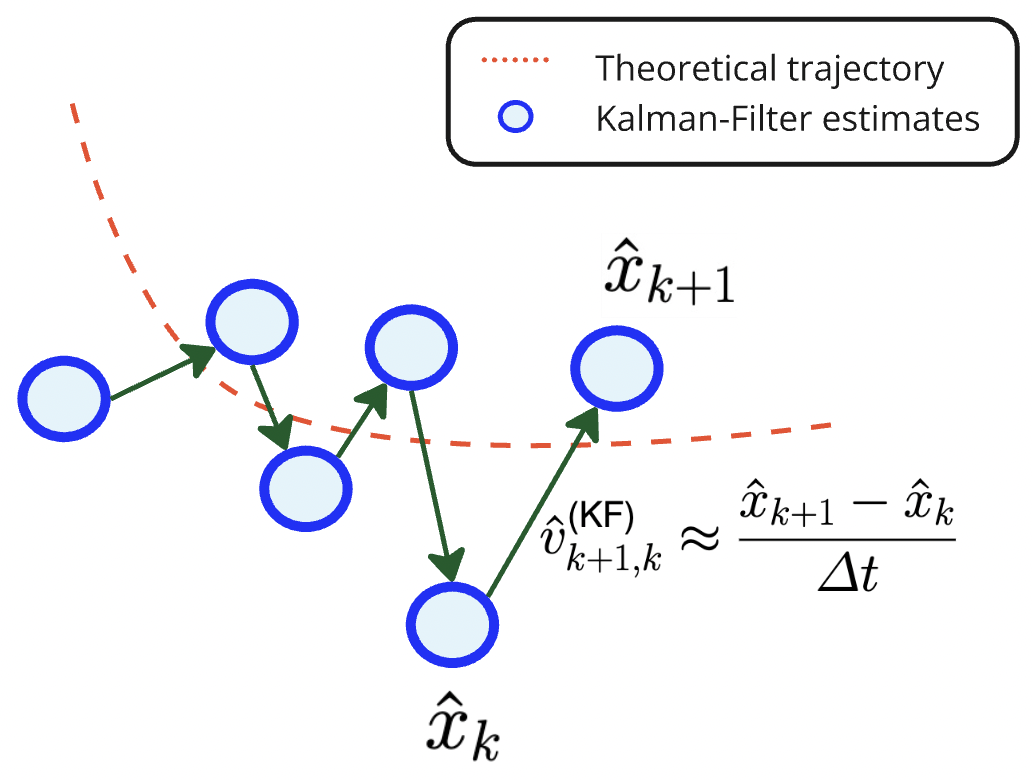
- Given the KF estimated positions, we can approximate the velocities, with the simple derivative.
- It is assumed that the acceleration is incorporated in each velocity step.
Estimating the Actual Kalman-Filter Velocity

The presence of noise is noticeable in the velocity estimates.
Estimating the actual Kalman-Filter velocity

Estimated KF velocities error
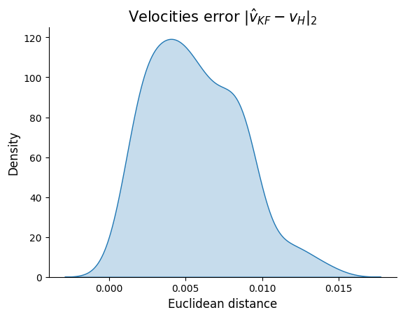
Estimated KF Velocities Error
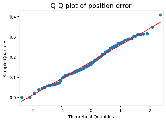
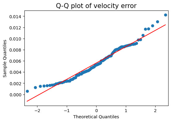
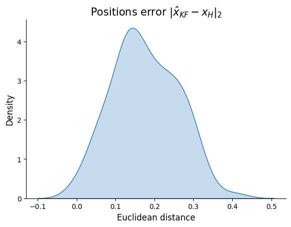
- D’agostino and Pearson normality test results for the position errors: \(\text{Test Statistic}=1.642\), and \(p=0.440\).
- For a significance value of \(\alpha=0.05\), we fail to reject H0, so we infer normality, since \(p>\alpha\).
Kalman-Filter: Simulation Parameters
\(A = \begin{bmatrix} 1 & 0 & \Delta t & 0 \\ 0 & 1 & 0 & \Delta t \\ 0 & 0 & 1 & 0 \\ 0 & 0 & 0 & 1 \\ \end{bmatrix},\) \(H = \begin{bmatrix} 1 & 0 & 0 & 0 \\ 0 & 1 & 0 & 0 \\ \end{bmatrix}\), \(\hat{x} = \begin{bmatrix} x_k \\ y_k \\ \dot{x}_k \\ \dot{y}_k \end{bmatrix} = \begin{bmatrix} x_k \\ y_k \\ v^{(x)}_k \\ v^{(y)}_k \end{bmatrix}\)
- \(Q = \sigma_Q^2 \cdot \mathbb{I}_{4 \times 4}\) (process noise, dynamics uncertainty)
- \(R = \sigma_R^2 \cdot \mathbb{I}_{2 \times 2}\) (measurement noise)
- \(P = \sigma_P^2 \cdot \mathbb{I}_{4 \times 4}\) (estimates uncertainty)
- with \(\sigma_Q^2 = 10^{-3}\), \(\sigma_R^2 = 0.5\), and \(\sigma_P^2 = 500\).
